Noise Reduction during embryonic development. STATPHYS 22 Satellite Meeting, Zanjan June 27- July 1.

Présentation au sujet: "Noise Reduction during embryonic development. STATPHYS 22 Satellite Meeting, Zanjan June 27- July 1."— Transcription de la présentation:

1 Noise Reduction during embryonic development. STATPHYS 22 Satellite Meeting, Zanjan June 27- July 1

2 Or, many of us wouldn't be here... Embryonic Development : How to get from one cell to an adult multicellular organism. Embryonic Development should be a very precise process despite all kind of noise and fluctuations...

3 Outline : 1. A little background on genes, transcription and developmental biology. 2. What are the problems with our current understanding of embryonic development ? 3. What are the practical problems and how the embryo overcome these ?

4 Background on gene transcription. Both computers and genes transcription machinery of cells are information processing units. They are however, organised around completely different lines.

5 The computer's hard disk is a linear array of bits. Each program occupies a specific interval. The position and length of all the files are stored in a special table. The operating system refers to this table each time it is asked to execute a program in order to know which exact array of bits to load into the memory. Information processing in computers :

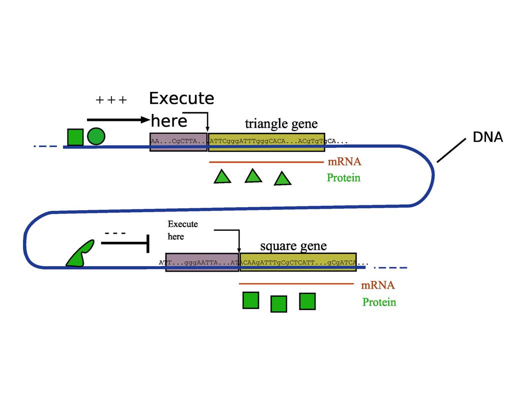
6 The Cell hard disk is its chromosome, which is a linear array of bases (A,T,C,G). The equivalent of programs are called genes. Each gene contains the manual to make a specific protein. Executing a program means reading a gene and copy it into RNA (transcription) and then send this RNA to a machine (ribosome) which will read it and make the protein (translation). There is no central operating system, no specific table which contains the position of the genes on the chromosome and their length. Information processing in living cells :

7

8 Gene products ( = proteins ) which control transcription of other genes are called transcription factor. They can either activate or inhibit a gene. [A] B prduction B A A B [A] B prduction

9 Transcription factors can group into complicated gene network A B C D E X Y S T Z Geneticists work, during the last 100 years, has been to uncover details of these networks in living organisms.

10 Background on embryonic dev. All cells have the same chromosomes, During the first stages of development, each cell, depending on its position inside the embryo, express a specific set of genes Kr Pdm1 Eagle

11 How do cells measure where they are inside the embryo ? How do they then decide which gene they have to express ? 0.250 mm 0.180 mm Fundamental question of Dev. Bio :

12 Morphogen Gradient ( >1900) Self-regulated (~1980 ) Two Main class of models :

13 Morphogene Gradient model ( Wolpert 69 ) There is a transcription factor with a variable concentration across the embryo. Cells switch ON/OFF the expression of some genes by reading this signal and comparing it to a given threshold. C in x threshold C out x If (C in > Threshold) Then express GeneA else don't express GeneA

14 Self Regulated models Modèles ( Turing 53 ) There is no need to break the symmetry with an outside signal, it can spontaneously bereak all by itself ! X Y

15 1987 : Bicoid is established as the paradigm of morphogens (Driever, Nusslein-Volhardt) 1989 and eve stipe 2 : Self regulated models are sent to trash.

16 bicoid is the dream gene, with all the properties people would have predicted : 1- The bicoid RNA, provided directly by the mother, is localised at the anterior pole.

17 2- The bicoid protein concentration gradient is established early and maintained.

18 3- bicoid protein is a transcription factor for all downstream gap genes (and many more) : – hunchback, – kruppel, – knirps, – giant, – eve...

19 4- Changing the gene's number of copy in the mother shifts expression domains in the embryo. [bcd] x hb x TheoryExperiment

20 The basics are then completely understood...... But what about precision ?

21 Precision: similarity between genes expression domain in different embryos.

22 A naive morphogene gradient model is too much sensitive to noise : x The initial gradient can vary from embryo to embryo. x The size of the eggs can vary. The environnement can vay.

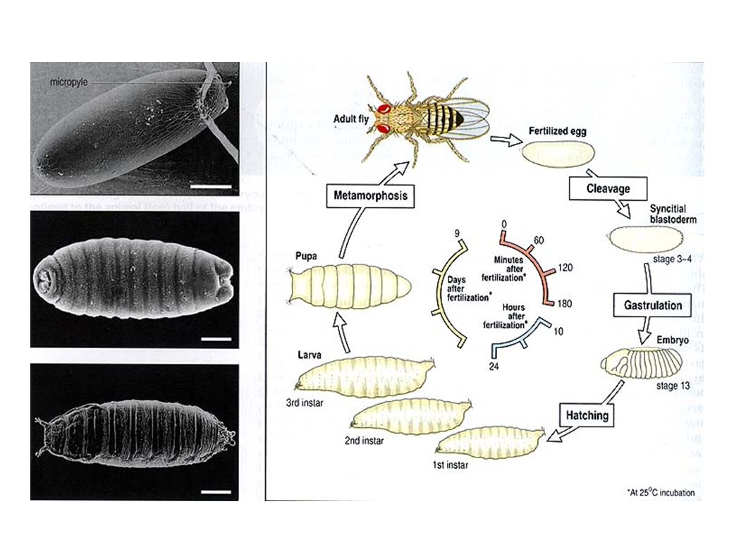
23 Do the experiments, and measure stuffs precisely,... In the model system for embryonic development : Drosophila melanogaster (fruit fly).

24

25 bcdnos hb kr kni gt ? evehairypaired maternel gap Pair rule Genetic network of the first stage of development.

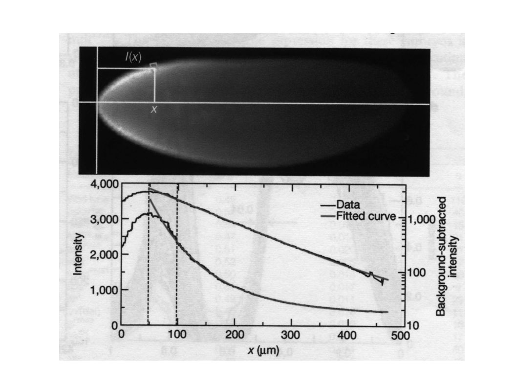
26 x I bcd hb kni Kr bcd hb Kr kni gt eve images de FlyEx (John Reinitz) 0.5 mm

27

28 0.1 E.L. Hill Coefficient : 10 ! If Bcd hb

29 What if we do the same measurements in >100 embryos ?

30 bcd is extremely noisy (Std dev of the positional information : 7% EL) But... hb extremely precise. (Std dev of the positional information : 1% EL)

31 Comparison between positional precision of bcd and hb expression domain.

32 Measuring the exponential decay of bcd gives the same results for its precision.

33 There is no correlation between the egg size and bcd positional information (r ~ 0). But the correlation between hb and the egg size is perfect (r= 0.82) ! bcd hb

34 No temperature variation effect ! bcd hb

35 OK, bcd is very noisy and does not know about the scale of the egg. Hb on the other hand is finally not very sensitive to the bcd, filters out all of the noise and make the signal proportionnal to the egg size. But.... Then what to do whith the Driever (and many others ) experiments on dosage modification of bcd ?

36 We may change our view if we measure stuffs precisely... bcd hb

37 OK... there are mechanisms which filter out the (huge) noise of the morphogene. maternal control ? Candidates : nos, caudal,torso,exu, staufen. zygotique control? ( Back to self-regulated models ? Candidates : Kr, kni, gt, runt, eve,...

38 To find the mechanism, we have to analyse the genetic network : program : induce a mutation, and look at the effect not only on the position of the hb domain, but on its precision.

39 Example : Kr 1- Stuhl has demontrated that hb regulates Kr (92) 2- Jackle has demonstrated that Kr mutation, shifts hb domain (86). bcd hb kr ? This is all we need to make a nice feed-backed, self correcting model !

40 Kr mutation has NO influence on hb, neither on its positon nor on its precision, which remain 1% !

41 None of the genes of the network (or outside the network ) has any effect on hb precision !

42 Mutating the maternal gene stauffen increases the error rate of hb to bcd level 7% !

43 Back to more trivial models ? What if we had two maternal gradients : one anterior (bcd) activating hb, one posterior (very hypothetical) inhibiting it? Bcd P (hyp) It works if the grads are correlated. 1- Hb position independent of Bcd noise. 2- Explain dosage modification experiments 3- Can compensate temperature variation. Bcd hb P

44 Conclusions : Introducing the concept of precision and use of quantitative methods in dev. biol. The bicoid as paradigm of morphogene dogma has to be revised. All the noise is filtered out in one step ! The real morhogene seems to be hb. Precision is under maternal control, via stauffen.

45 Stanislas Leibler (Rockefeller University, New York) Eric Wieshaus (Princeton University, New Jersey)

46 Eves stripes rules or how the turing models where discarded.

47 Simple gradient model. Activator : exp (-x/k) ; needs threshold t Hb position : x = k log(1/t) Shift in Hb in with n dose bicoid : dx = k log(n) Anterion and Posterior gradient model. Activator : exp (-x/k) ; Inhibitor exp ((x-1)/k) Hb Position : x = ½ (independent of k ) Shift in Hb in with n dose bicoid : dx = (k/2) log(n)

48 2- Aggrégation et Ecologie « neutre ».

49 Aggregation d'organism induit par le bruit stochastique des morts et des naissance. Ou Comment les simples alea de la naissance peuvent induire les espèces à s'agglomerer, et ceci sans faire appel à une quelconque attraction social entre les individus.

50 Prenons un ensemble d'organismes qui se dupliquent (avec un taux ), meurent (avec un taux ) et diffusent (avec un coef D). L'équation d'évolution de la concentration de ces bactéries est : Si les taux de mort est de naissance sont égaux ( ), la diffusion tend à homogénéiser le milieu.

51 La simulation « discrète » des bactéries a un effet exactement contraire : A chaque pas de temps dt 1- Chaque bactérie décide au hasard, avec une proba dt (<<1), si elle se duplique ou si elle meure. 2- Chaque bactérie effectue un mouvement brownien. La diffusion ne peut pas empêcher l'agglomération, quelque soit son importance ! Modèle proposé pour expliquer l'agglomération des plankton à la surface de l'Ocean.

52 L'erreur vient de l'ecriture même des équations continues. En écrivant ces équations, qui concernent des quantités moyennes, on suppose que les fluctuations sont faible. Cette hypothèse peut-être grossièrement violée !

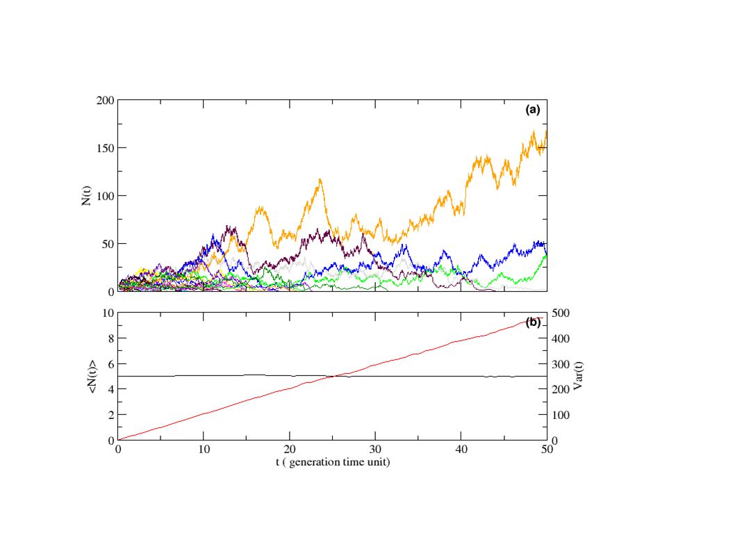
53 Prenons un système à ZERO dimension, un ensemble de bactérie avec le même taux de mort et de duplication. La probabilité, pour que le système, pendant un temps dt, passe de taille n à n+1 ou n-1 est Si le système tombe à 0 individu, il ne s'en sort plus.

54

55 Equation maîtresse : Les moments :

56 Pour d > 0, il suffit de disposer des boites d'organismes le long d'un réseau à d dimensions. Chaque boite est soumis à : (i) les fluctuations interne de mort et de naissance ; (ii) fluctuations dues à la diffusion.

57 La moyenne reste constante :

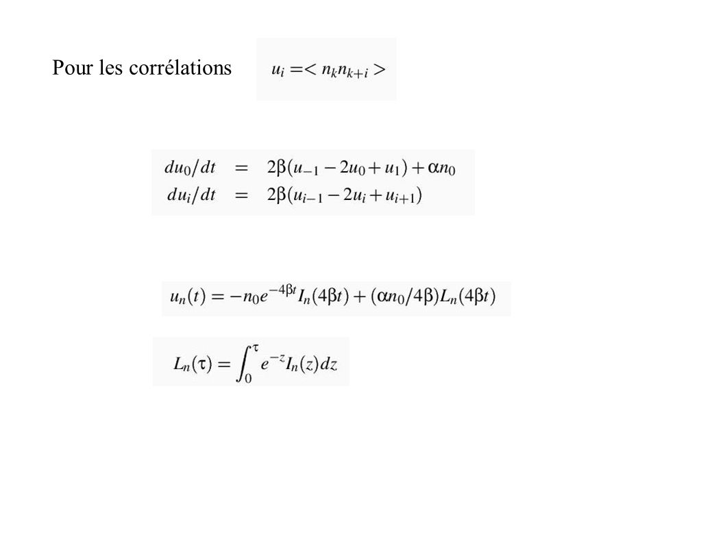
58 Pour les corrélations

59

60 Les corrélations divergent avec le temps si d 2

61 Les individu s'auto-organisent en cluster pour d=1 ou 2 et la taille des clusters croit comme si d=1 si d=2 A trois dimension, la croissance illimité d'aggrégats disparaît.

62 Le simple bruit stochastique discrète des morts et naissance peut provoquer le phénomène d'organisation en aggrégat, sans qu'on ait besoin d'invoquer des interactions non-linéaire/sociale

63 Mais ce modèle est beaucoup trop simpliste Les taux de mort et de naissance ne peuvent pas être indépendants de la densité : si il y a trop de monde autour d'un organisme, les ressources localement disponible sont vite épuisé, et l'organisme ne pourra pas se dupliquer.

64

65 Hypothèses du modèle de Hubell : Toutes les espèces (d'un même niveau trophique) sont strictement équivalent : même taux de mort, de naissance, de migration,... L'espace est saturée : il faut qu'un individu meure pour qu'un autre puisse se dupliquer. La place libéré par la mort d'un individu peut-être prise par le descendant de n'importe quel individu ( encore vivant ) appartenant à n'importe quel espèce.

66 Considérons une espèce parmis d'autre :

67 A d=0, Proba pour que l'espèce A passe de n à n+1 : Proba pour qu'un individu d'un autre espèce meure Proba pour qu'un individu d'espèce A se duplique. J : nombre total d'individu (quelque soit l'espèce) dans l'écosystème (fixe).

68 A d=0, Proba pour que l'espèce A passe de n à n-1 : Proba pour qu'un individu d'un autre espèce se duplique Proba pour qu'un individu d'espèce A meure. Si n=0, il n y a plus d'évolution : l'espèce est éteinte. Si n=J, il n y a plus d'évolution : l'espèce est dominant.

69 On peut, par les même procédés, généraliser à d dimension, et extraire les corrélations :

70 Solution exacte Approx temps long

71 Les organismes de chaque espèce s'auto-organisent en cluster pour d=1 ou 2 et la taille des clusters croit comme si d=1 si d=2 Si suffisemment de temps est accordé, un seul espèce dominera tout l'écosystème ! Cette tendance doit être nettement plus marqué dans les écosystèmes 1d (les lits des rivières, le long des plages,...) quand dans les 2d (la plupart des écosystèmes).

72 A d=3, un équilibre s'établit, les corrélations décroissent en ~1/r, Le système ne contient plus d'échelle charactéristique.

73 La domination aux temps long par une espèce est limité par L'échelle des changements climatiques L'échelle des mutations. Combien d'espèce présents dans l'écosystème ?

74 Conclusions : L'aggrégation est une conséquence des aleas de mort et de naissance. Les intercations sociales, les niches écologiques... peuvent bien sûr exister, mais leurs importance doit être mesuré à l'aune de l'étalon neutre.

75 3- Intéraction prédateurs-proies

76 La nature est dominé par les intéractions prédateurs-proies, parasite-hôte, pathogène-hôte. ces intéractions forment des chaines alimentaires

77 Peut on comprendre la dynamique de ces populations ? Savoir si une chaine alimentaire est stable ? Prédire l'influence des perturbation qu'on y apporte ?

78 Plus modestement, peut on comprendre la dynamique d'une espèce de prédateur et d'une espèce de proie ? Lotka et Voltera, 1930 :

79 Le modèle de Lotka-Voltera souffre de plusieurs défauts : Il est marginalement stable. Le bruit stochastique provoque l'extinction. Il n'est pas spatial : n'importe quel prédateur a accèse à n'importe quel proie. N'a jamais été vraiment observé !!!

80 Construire un écosystème modèle : Spatialement étendu Temporellement long ( ~ 100 générations ) Où tout les paramètres sont mesurables Et qui permet de constituer des statistiques significatifs. Espèce microbienne (prédateur : Dyctiostelium, proie Klebsiella) à temps de générations rapide

81 Microbes Fluorescentes (GFP,RFP,...) Petri dish spatialement infini (60 mm) Microscope automatisé et analyse d'image Carte spatio- temporelle des deux populations.

82 A court terme, étudier : l'influence des fluctuations le rôle de l'espace A plus long terme, Ajouter d'autres niveaux trophique.