NANCY 09-06-05 D. Calogine K.Chetehouna E. Lamorlette J. Margerit S. Ramezani N. Rimbert O. Séro-Guillaume Modèles de Combustion en milieux poreux Caractérisation.

Présentation au sujet: "NANCY 09-06-05 D. Calogine K.Chetehouna E. Lamorlette J. Margerit S. Ramezani N. Rimbert O. Séro-Guillaume Modèles de Combustion en milieux poreux Caractérisation."— Transcription de la présentation:

1 NANCY 09-06-05 D. Calogine K.Chetehouna E. Lamorlette J. Margerit S. Ramezani N. Rimbert O. Séro-Guillaume Modèles de Combustion en milieux poreux Caractérisation de la végétation Modèles de propagation à grande échelle Modélisation de la lutte par largage

2 INTRODUCTION

3 The Scales Scale of Combustion Flames above vegetation Convection Radiation The wood is a porous medium with several phases and several components Scale of “chemical” reactions: Pyrolysis Drying Scale of Combustion Convection Radiation The vegetation is a porous medium with two phases

4 The modeling at different scales lvlv Vegetal Phase air + gaz Phase Mesoscopic scale Macroscopic scale 10 < Re < 10 4 Porous medium combustion model Gigascopicc scale 10 7 < Re Propagation model

5 VEGETATION MODEL

6 Vegetation Model CIRAD Software A.M.A.P. Vegetation has been considered as fractal Dedicated to virtual Agronomy Not well suited for computational purposes

7 Vegetation Model Construction by Iterated Functions Systems I.F.S. Barnsley, Hutchinson Deterministic Probabilistic p i probabilites Probabilityis p i

8 Example Vegetation Model Calogine et al. 1998

9 Vegetation Model Model 1 Order : 7 Model 2 Order : 4 Model 3 Order : 5 Other Types of Vegetals

10 Vegetation Model

11 Automatic generation of the mesh

12 7 millions cells h=10m Vegetation Model

13 écoulement z x yExperiment I.F.S. (order) NxNxNxNx NyNyNyNy NzNzNzNz N x xN x xN z tttt Simulation 1 6 ( loc =4) 171129171 3 772 089  t  0,1 Simulation 2 5 ( loc =7) 1812x90181 5 896 980  t  0,08 Simulation 3 5 ( loc =9) 2322x116232 14 884 450  t  0,06 Simulation n 7 (14) 501501501 125 751 501  t  0,03

14 Vegetation Model

15 FIGHTING MODEL

16 Dropping model Continuous Eulerian model Continuous Eulerian model New equation for Interfacial area density New equation for Interfacial area density New closure for Interfacial velocity New closure for Interfacial velocity Averaging procedure

17 Dropping model Stochastic approach Stochastic approach Figure 1: fitting of the drop spray p.d.f. V SL = 0.041 m/s V SG = 35 m/s. From left to right the p.d.f. are log-stable p.d.f., Upper-limit Evans p.d.f., log-normal p.d.f. and log-Weibull p.d.f. Log-Levy stable distributions are better distributions than the usual ones

18 Dropping model Transport Equation for the interfacial density It can be shown that: It can be shown that: Where S c is a source related to curvatureWhere S c is a source related to curvature S e is a surface stretching termS e is a surface stretching term S fc is a term related to fragmentation and coalescenceS fc is a term related to fragmentation and coalescence

19 Dropping model Two –Fluids Model Mass Balance MomentumBalance Closure Equations Supplementary Constitutive Laws

20 Dropping Model 4.8 million cells used for the atomisation stageA 850,000 cells grid used in the dispersion stage

21 Dropping Model velocity field around the cloud of retardant in the airplane frame of reference t = 0.5 s isosurface a = 0.5 (2% gum mass percentage)

22 Dropping Model The results of part I are initial conditions for part II Data aliasing and averaging From atomisation modelling to spreading modelling

23 Dropping model Dropping Simulations

24 A 3D DETAILED MODEL OF COMBUSTION

25 Write all equations at Microscopic scale using distribution theory, so that boundary conditions are included in the equations. Example : Mass Balance in the gaseous phase Albini Model at microscopic level (1985) First Step: Extension of the equations Homogenized Medium

26 Convolute the equations with a compact support kernel of size h denoted m. In the gaseous phase Balance of Mass Balance of momentum Balance of Energy In the vegetal phase Balance of Mass Balance of Energy Second Step: Average procedure

27 Homogenized Medium For example And we define the following Average Quantities From the Balance of Momentum in the gaseous phase we obtain the relation Is the porosity

28 Homogenized Medium At Step 2 several new quantities has been defined. They must be related to average variables: It is the Closure operation. We used Rational Extended Thermodynamics (R.E.T.) Or Extended Irreversible Thermodynamics (E.I.T.) Jou, Casas-Vazquez, Lebon Third Step: Closure operation Equations for these new quantities are obtained by writing that the entropy production is positive. Müller, Ruggeri

29 Homogenized Medium The obtained model is very general and has the following characteristics 1°) Two Temperatures, one for each phases with a modified Fourier law 2°) Contains a model of pyrolysis for the vegetal with relaxation times 3°) The vegetal phase has an internal structure with possible modelling of chemical actions of retardant 4°) Extended Navier Stokes equation, with memory

30 Homogenized Medium Several Simplifications can be Made 2 Temperatures1 Temperature Generalised Fourier LawUsual Fourier Law Instantaneous momentum Transfer between Phases...

31 Homogenized Medium Energy Balance Mass Balance Solid Constituents Liquid Constituent Gaseous Constituent Mass Transfer Between Phases “wood and air” Simplified 3D Model PHASE W AS WOOD

32 Homogenized Medium Energy BalanceMass Balance Mass Transfer Between Phases “wood and air” 3D Model Continued PHASE F (AS FLUID) GAS Balance of Momentum + Thermodynamics Relations +Radiative Transfer Equation

33 15m 9m 6m 25cm Distribution exponentielle de porosité 1m/s Heat flux Bilan de quantité de mouvement Phase gazeuse Bilan d’énergie Litière+Gaz Bilans de masse Litière+gaz Équation du transfert radiatif Litière+Gaz Cinétique Chimique Litière +Gaz HH liti è re Numerical experiment in fire tunnels

34 AVI Numerical experiment in fire tunnels

35 A 2D PROPAGATION MODEL

36 Propagation Modeling Reduction 3D Combustion 2D Propagation Hypotheses Vegetation Height  small compared to the gigascopic scale “Gigascopic Scale L” Flow Almost Parallel to the ground

37 Propagation Modeling The Ratio  L<< 1, Small parameter L can be the size of the fire or the distance to the fire front Outer Part of the Asymptotic Expansion Inner Part of the Asymptotic Expansion = Propagation Model Quantities are continuous across the vegetation toward ambient air Use of Matched Asymptotic Expansion on the Whole Domain z > 0 (vegetation +ambient air) Asymptotic Expansion Asymptotic Expansion

38 Propagation Modeling Model I Only for phase W Propagation Model Are quantities deduced from experiments… outer expansion Mass Balance for the cellulose Mass Balance for the char… Energy Balance Radiative flux Temperature of gases Mass Balance for the water…

39 Avant le front d’évaporation Zone IDans la zone de séchage, Zone IIEntre la zone de séchage et la zone en feu, Zone IIIDans la zone en feu, Zone IV Dans la zone brûlée, Zone V Propagation Modeling

40 Modélisation de la Propagation Takes into account Drying, Pyrolysis, Wind, Slope Radiative flux with Is the inclination of the flame and K is the extinction function

41 Zone I Zone III Zone IV Zone V Zone II Highly non linear 5 free boundaries Propagation Modeling

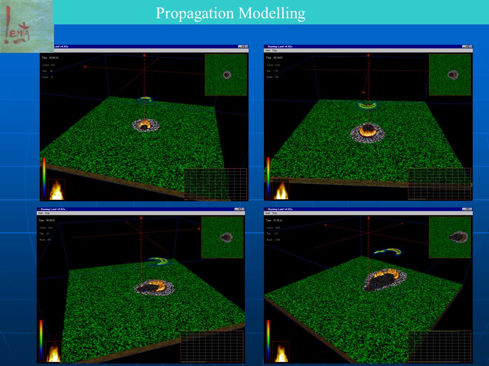
42 Occupation density 0.5Moisture 0.07 Propagation Modelling

43

44 Wind effect, 30 mn, 45 mn, 1h15, 1h50 Propagation Modelling

45 Under a certain value of the occupation density the fire will not propagate Percolation Density : Propagation Modelling

46 FIGHTING MODEL

47 PESPECTIVES

48 Travail en cours Caractérisation de la végétation comme milieu poreux. Thermique et Radiatif Modèle de flamme dans le modèle de propagation Rendre opérationnel le modèle de propagation à très grande échelle. Amélioration de la convection. Pris en compte de l’effet du retardant sur la propagation Modèle simplifié de largage

49 NANCY 09-06-05

50 Travail en cours

51 Level Set or V.O.F. Formulation

52

53 What happens if the initial density is decreased ? Control on the initial density Simulation

54 3 QUESTIONS OF OPTIMIZATION AND CONTROL

55 What happens if the initial density is decreased ? Control on the initial density Simulation

56 Au dessous d’une valeur critique de de la densité d’occupation le feu ne se propage plus. Densité de Percolation : Propriétés à basse densité Expérience de Propagation-Percolation Fractalité du front ?? Mécanismes mis en jeu ??

57 Question 1: Fire Front Reconstruction Data Assimilation Is it possible to find a initial distribution of vegetation and a T>0 such that: Prevention for?

58 Aerial fighting by indirect attack The dropped fluid = Water + Ammonium Phosphate + Gum The Ammonium Phosphate decreases the activation energy in the pyrolysis law : Control on the retardant distribution Simulation

59 Fire Front Reconstruction Data Assimilation The flame is defined by: height tilt angle emitted power rate of spread

60 2°) Que se passe-t-il si la densité de combustible tend vers 0 ? Fire Front Reconstruction Data Assimilation Flame model0.741.55 0.771.48 0.801.41 1.750.831.35 1078.50.861.29 0.170.891.23 3.6 %0.921.16

61 Fire Front Reconstruction Data Assimilation Burnt zone Burning zone Unburnt zone. Extinction line Fire line Flux meters positions Data from satellite?

62 1 QUESTION OF STABILITY AND UNICITY

63 Uniqueness and stability. Let  the characteristic function of the burning zone

64 Uniqueness and stability. For homogeneous conditions of vegetation the straight line seems to be the only stable solution (Depend on wind and slope) The direction of propagation seems to be along the line of maximum rate of spread

65 f(T) une fonction non linéaire Wave solution Rate of spread is solution of the non linear egeinvalue problem Problème qui peut avoir plusieurs solutions ou pas du tout Rate of spread.

66 Dimensional analysis Small parameter Rate of spread. We look for a series solution

67 Radius of convergence of the series and uniqueness ? Rate of spread. is the unique solution of

68 1°) Much more questions than answers Conclusion 2°) Mathematicians are welcome 3°) Thank you

69 TYPOLOGIE DES MODELES

70 Modèles Géométriques Méthode de Enveloppes Hypothèse sur la forme géométrique du feu Méthode de construction du front à t + dt Méthode qui marche bien mais fournit des solutions très régulières

71 Modèles empiriques Modèle de Rothermel s surface spécifique, d épaisseur couverture végétale C charge ducombuxtible sec, r masse vol. sec. D H chaleur contenue dans la particule sèche V vitesse du vent à mi hauteur tan j pente Hu Humidité des particules de combustible He Humidité d’extinction R = f( s, d, r, tan j, D H, V, Hu, He) R = vitesse de propagation Hypothèse Chaque partie du front est déplacée avec la vitesse normale R P P+Rndt Front à l’instant t Front à l’instant t+dt n Méthode qui marche bien mais fournit des solutions très régulières

72 Modèles Physiques Modèle de Réaction diffusion Prototype Equation seule (1) Système d’Equations (2) Réactions chimiques Dynamiques des populations Modèles dits Physiques ont la structure

73 COMPARAISON DES MODELES

74 Modèles de Réaction diffusion peuvent faire aussi bien que les modèles d’enveloppe et de Rothermel Résultat des Courses Rothermel Ellipses Hamilton Jacobi Réaction- Diffusion Les modèles d’enveloppe se comportent très mal à basse densité ?

75 Conclusions 1°) Les modèles de propagation dits de Réaction-Diffusion pourraient fournir plus d’information que les modèles semi empiriques. 2°) Théoriquement ils peuvent faire au moins autant que les modèles d’enveloppe ou de type Rothermel. 3°) Ils sont plus faciles à calibrer Questions 4°) Peuvent ils faire plus ? Et rendre compte de comportements très irréguliers du front de flamme 5°) Si oui quelle stratégie de modélisation ? Conclusions partielles

76 Stratégie de Modélisation Modèle « Détaillé » Réduction Modèle « Souhaité » Sous modèle 1Sous modèle 2 Sous modèle N … Complexification Spécifications Echelle Objectifs…