La mesure de l’eau dans l’atmosphère

Présentation au sujet: "La mesure de l’eau dans l’atmosphère"— Transcription de la présentation:

1 La mesure de l’eau dans l’atmosphère
Pluviomètre à Auger Radiosonde humidité GPS – Tomography Weather Radar Micro-wave T and H20 Raman Lidar Des observations « temps réel » pour la prévision immédiate principalement Des observations ciblées sur les évènements extrêmes

2 La mesure de l’eau dans l’atmosphère
Radiosonde humidité Hygristor résistif (carbone)

3

4

5

6

7

8

9

10

11

12 Geodesy and Geodynamics Lab Institute of Geodesy and Photogrammetry
GPS Tomography GPS-Tomography: Determination of the spatial distribution of water vapor using the GPS navigation satellites Dr. Marc Troller Geodesy and Geodynamics Lab Institute of Geodesy and Photogrammetry ETH Zürich

13 Tropospheric path delay DPD using GPS
n: refractivity index s : signal along W s0: Signal along W0 for geodetic applications Error dry wet for climate and atmospheric research Signal

14 Mathematical relations: GPS meteorology
: wet path delay : conversion factor depends e.g. of the day and station coordinates : Precipitable water vapor: Vertically integrated mass of water vapor per unit area [kg/m2] : wet refractivity : specific humidity [kg water / kg air] : specific gas constant for dry air

15 Automated GPS network (AGNES) of swisstopo
30 AGNES stations 48 additional stations AGNES height range: 400 m (FHBB) - 3‘600 m (JUJO) AGNES stations Other stations

16 Numerical weather model aLMo
Alpine Model aLMo: Implementation of the non- hydrostatic local weather model COSMO for Switzerland Operational at MeteoSwiss since April 2001 385x325 grid points (horizontal spacing ~7km), 45 vertical levels © MeteoSwiss Operational domain and orography of aLMo

17 Evaluation of path delay modeling with the AGNES network
aLMo: numerical weather model AGNES: GPS determined PD Saastamoinen: Standard model according to Saastamoinen, 1972

18 Film 3x

19 Principle of GPS-tomography
Determination of the distance between satellite and receiver: ni: Constant refractivity in voxel i Dsi: Signal length in voxel i k: Number of voxels using a voxel model: r: Signal n: Refractivity index

20 Medical vs. GPS-tomography

21 Tomography using GPS double-difference observations
One double-difference: : Slant distance from station a to satellite i

22 GPS-tomography using AGNES
wet refractivity [ppm] height [m] GPS-tomography using AGNES

23 Weather Radar Dr. Urs Germann Locarno Monti MeteoSwiss

24 reddish colours > 40mm/h
Weather Radar reddish colours > 40mm/h 300 km

25 reddish colours > 40mm/h
72 automatic gauges reddish colours > 40mm/h 300 km

26

27 Prolog A weather radar is the only instrument that provides
in real-time a three-dimensional picture of precipitation at a high spatial and temporal resolution (1 km, 5 min) over a large range of intensities (drizzle to hail) up to a maximum range around 250 km (?). But a lot of work is needed, and many problems remain unsolved.

28 Radar: - 400km diameter - 5min, 1km - indirect measure-ment of precip
1 satellite 1 radar 72 gauges 300 km Courtesy: I Giunta infrared red colours > 40mm/h MSG: - continental scale - 15min, 5km - no direct observation of precipitation Radar: km diameter - 5min, 1km - indirect measure-ment of precip Gauge network: m scale - 10min, 25km - direct measure-ment of precip

29 Frequencies Frequency wave-length band meteorological application
MHz 1-15 m VHF wind profiler and ocean surface motion MHz m UHF wind profiler 1 GHz 0.3 m L-band boundary layer wind profile 2-4 GHz 7-15 cm S-band long-range precipitation radars 4-8 GHz 4-7 cm C-band 8-16 GHz 2-4 cm X-band precipitation radars, marine radars 16-20 GHz 1-2 cm Ku-band radars 35 GHz 8.5 mm Ka-band precipitation and cloud radars GHz 3 mm W-band cloud radars, Mie minimum

30 How does a weather radar work?
tau = pulse length (s) lambda = wavelength (cm) f = frequency (GHz) PRF = pulse repetition frequency (kHz)

31 STALO stable local oscillator
radome scattering objects antenna 250 kW low-noise amplifier duplexer minimum detectable signal (depends on receiver noise): dBm receiver transmitter STALO stable local oscillator

32 What does a weather radar measure?
A weather radar can measure several different quantities: the radar reflectivity (related to precipitation rates) the Doppler phase shift (related to radial component of wind vector) polarimetric quantities (related to shape and orientation of raindrops)

33 Radar pulse volume pulse length tau (typically 0.5 μs)
radial resolution Δr = c tau / 2 (typically 75 m), where c is speed of light. 3dB beamwidth beta = 70 lambda / D (typically 1deg), where lambda is wavelength and D is antenna diameter. pulse volume V = π r2 beta2 c tau / 8 (r2 dependence!), where r is range from radar (3dB beamwidth!).

34 Refraction Refractivity N of air depends on pressure p, vapor pressure e and temperature T. Assume that p, e and T only depend on height, then, radar rays lie on circles. To account for refraction we introduce an effective earth radius reff (not displayed in the figure). With true earth radius r we have k = reff / r = 1 / (1 + r dN/dz 10-6) Working with reff radar rays become straight lines. For standard atmosphere and heights below 1 km we have dN/dz = - 40 km-1. Using this decrease of refractivity with height we get k = 4/3 r

35 Elimination of non-meteo echoes (clutter)
no elimination elimination on

36 Scatterers: examples daily total of residual clutter, partly airplanes
all clutter, elimination OFF Clutter = all non-desired echoes precipitation

37 Sensitivity saturation
Minimum detectable signal (depends on receiver noise): typically -110 dBm Dynamic range: typically 90 dB signal of precipitation signal power receiver noise distance

38 Sensitivity diagram of Monte Lema radar
rainfall 10mm/h: beyond 230 km saturation drizzle 0.2mm/h: up to 200 km clear-air turbulence: up to 4.5 km 1 mosquito: up to 600 m receiver noise Germann, 2000

39 Very strong echo (hail ?)
echoes above 55 dBZ, possibly hail plan view vertical cross section

40 Very strong echo (hail !)
plan view vertical cross section

41 Attenuation by water on radome
rain at radar site Germann, 1999

42 Summary

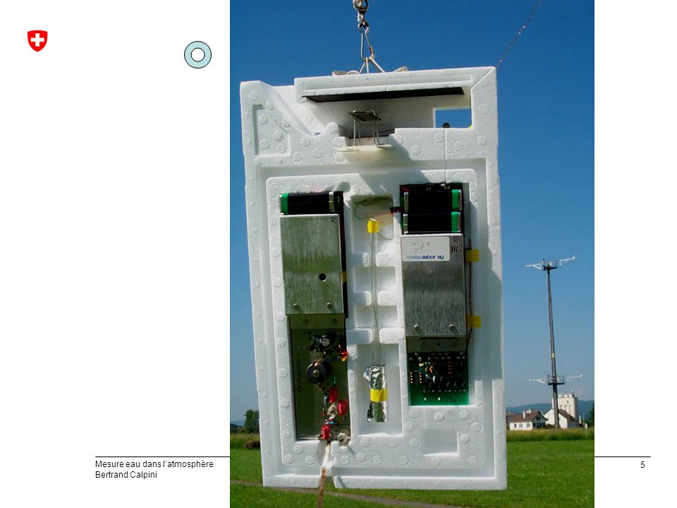
43 Passive Radiometer Mesure de l’extinction induite par le contenu en eau dans l’atmosphère: mesure « passive » Boundary layer profiles 1 profile every ~5 minutes Moving averaged over 12 samples (1 hour) daily plots

44 Spectral bands of operation:
Frequencies Humidity Profiling: GHz Band (7 channels) Temp. Profiling (Trop.): 50-59 GHz Band Temp. Profiling (BL): 54-59 GHz Band (4 channels) LWP / IWV: 23.8 / GHz 23.8 GHz 36.5/31.4 90.0

45

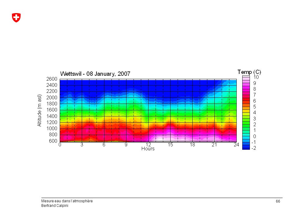
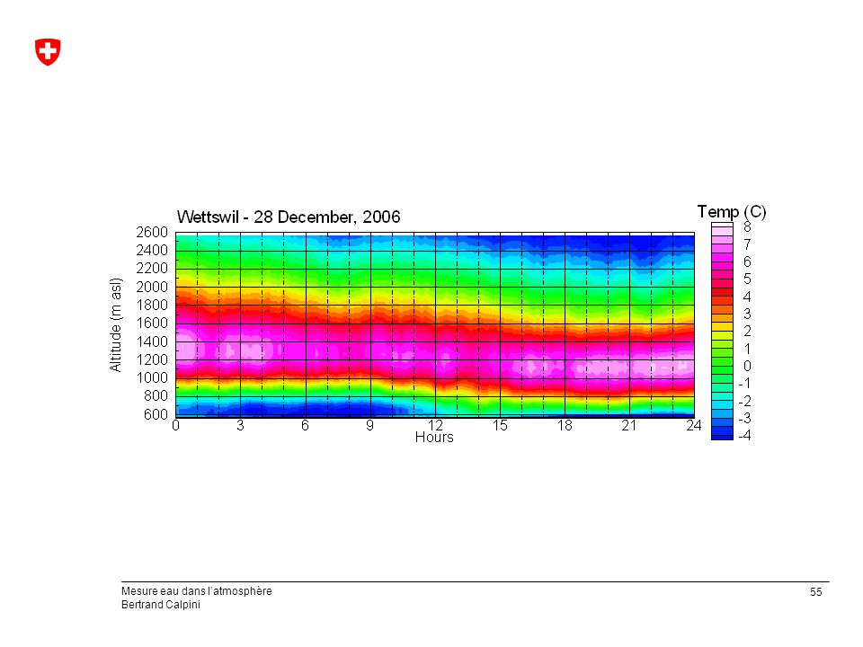
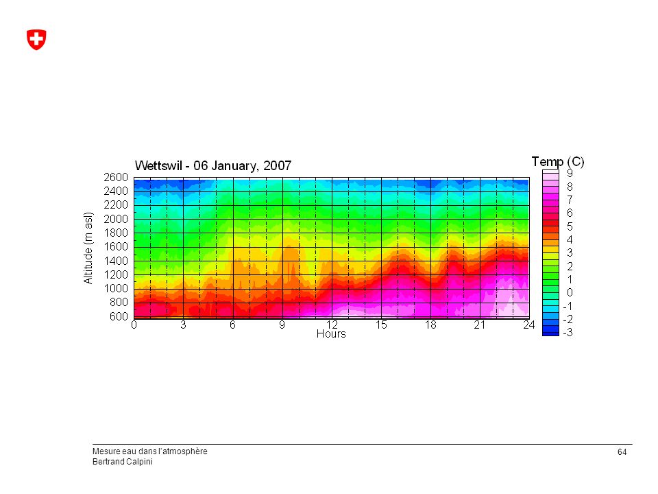
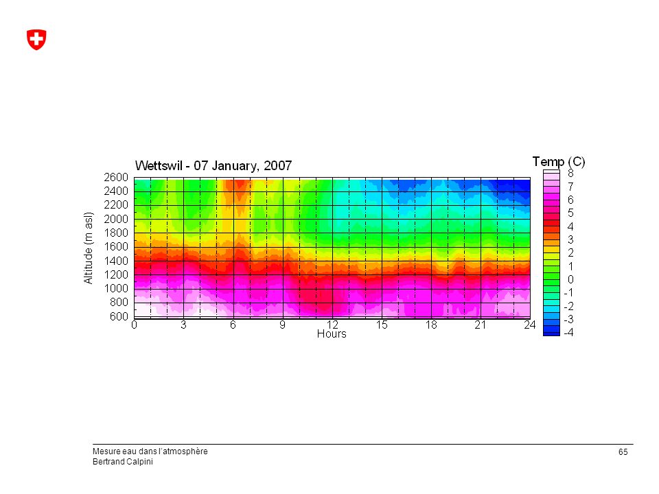
46 Wettswil (AWEL) Microwave radiometer for automatic temperature profiling and presence of precipitation Boundary layer profiles 1 profile every ~5 minutes Moving averaged over 12 samples (1 hour) daily plots

47

48

49

50

51

52

53

54

55

56

57

58

59

60

61

62

63

64

65

66

67

68

69

70

71

72

73

74

75

76