J. Duchesne1, P. Raimbault2 and C. Fleurant1

Présentation au sujet: "J. Duchesne1, P. Raimbault2 and C. Fleurant1"— Transcription de la présentation:

1 J. Duchesne1, P. Raimbault2 and C. Fleurant1
Etude de la morphométrie des arbres par combinaison de la géométrie fractale et de la physique statistique J. Duchesne1, P. Raimbault2 and C. Fleurant1 1. UMR 105 Paysages et biodiversité 2. UMR SAGAH

2 Une loi universelle de la morphométrie des arbres ?
Introduction Démonstration de la loi Résultats et discussion Conclusion

3 Une loi universelle de la morphométrie des arbres ?
Introduction Démonstration of the law Résultats et discussion Conclusion

4

5

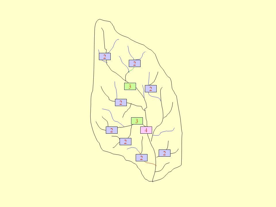
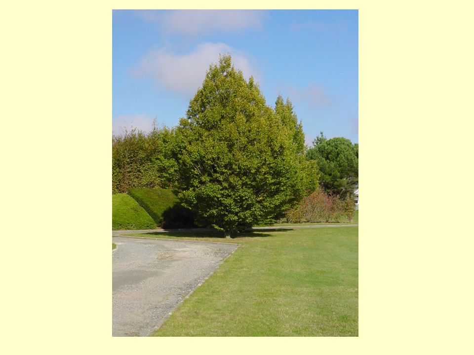
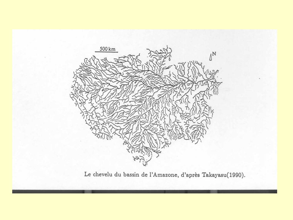
6 Réseaux hydrographiques Arbres
Ont en commun l’invariance d’échelle Structures fractales ramifiées

7 2 2 3 2 2 3 2 4 2 2 2

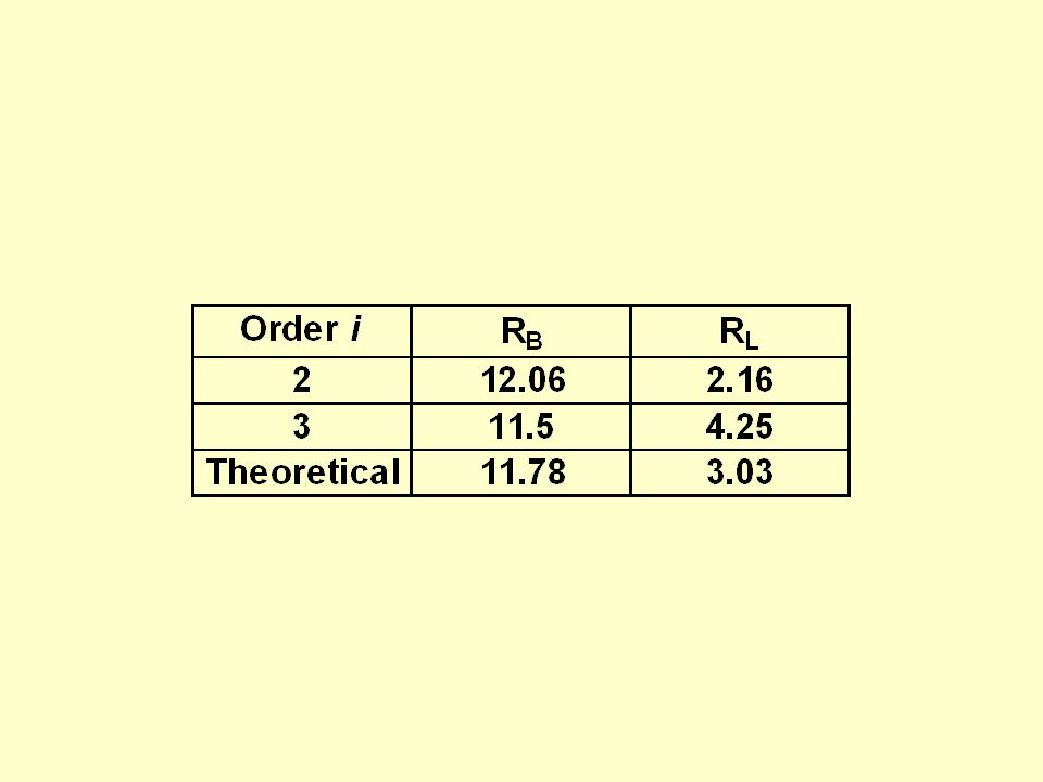
8 RC : rapport de bifurcation
N1 : nombre de tronçons du 1er ordre N2 : nombre de tronçons du 2ème ordre ……….. Ni: nombre de tronçons d’ordre i Rapports N1/ N2, N2/ N3, … Ni/ Ni+1 sont constants et notés RC : rapport de bifurcation

9 RL : rapport de longueur
: longueur moyenne des tronçons d’ordre 1 : longueur moyenne des tronçons d’ordre 2 ……….. : longueur moyenne des tronçons d’ordre n Les rapports L2/ L1, L3/ L2, … Li+1/ Li sont constants et notés RL : rapport de longueur

10 Ces deux résultats sont la marque d’une structure fractale ramifiée

11 Une loi universelle de la morphométrie des arbres ?
Introduction Démonstration of the law Résultats et discussion Conclusion

12 d’utiliser un raisonnement de physique statistique
Nous proposons d’utiliser un raisonnement de physique statistique

13 Une loi universelle de la morphométrie des arbres ?
1. Introduction 2. Démonstration de la loi Choix de l’espace symbolique

14 Symbolic space of Maxwell : the space of speeds
vz vy dvz dvy dvx vx

15 d3N is the number of molecules which the speed vector
ends to the elementary volume dvx dvy dvz , among a total number of molecules N

16 The two hypotheses of Maxwell
the independence of the 3 speed components ; the isotropy of the speed directions

17 The independence of the 3 speed components involves :
So, the 3 variables are separated

18 The isotropy of the speed directions is a natural hypothesis because
one can hardly imagine that some directions be privilegied The distributions f1, f2, f3 have the same form :

19 are sufficient conditions to determine the function F(v)
The two hypotheses of Maxwell are sufficient conditions to determine the function F(v)

20 Analogy between thermodynamics and natural networks
Maxwell approach Our approach

21 Notion of speed vector module Notion of hydraulic length
Analogy ... thermodynamics natural networks Notion of speed vector module Notion of hydraulic length v L

22 Analogy … thermodynamics natural networks
Maxwell approach vz vy dvz dvy dvx vx

23 Analogy … thermodynamics natural networks
Our approach L = l1 + l2 + l3 +… + ln

24 Analogy … thermodynamics natural networks
There are two differences between the two approaches ...

25 Analogy … thermodynamics natural networks
first difference : In thermodynamics In natural networks there are 3 components there are n components

26 Analogy … thermodynamics natural networks
• • •

27 Analogy … thermodynamics natural networks

28 Analogy … thermodynamics natural networks
second difference : In thermodynamics In natural networks the 3 components have the same mean the n components have not the same mean

29 Analogy … thermodynamics natural networks
• • • • • •

30 Analogy … thermodynamics natural networks
• • •

31 Analogy … thermodynamics natural networks

32 Maxwell’s two hypotheses
the independence of the 3 speed components ; the isotropy of the speed directions become the independence of the n length components ; the isotropy of the directions of the symbolic space

33 The Maxwell function becomes

34 The Maxwell results for f
And the same for vx, vy, vz become become

35 Une loi universelle de la morphométrie des arbres ?
Introduction Démonstration of the law Résultats et discussion Conclusion

36 … it is necessary to respect two conditions
which are strongly related to the statistical physics : 1. the size of the system much be very large compared with the elementary constituent which will be taken into account 2. the local properties of the system must be homogeneous

37 A large number of elementary constituents
Homogeneity of the population

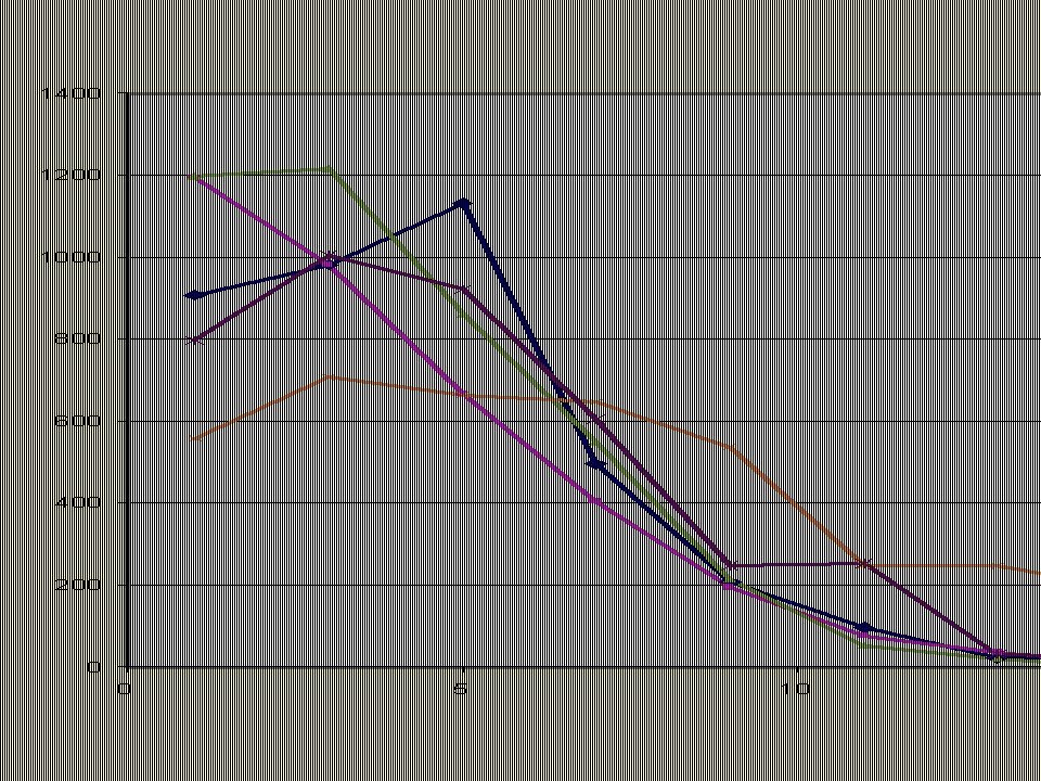
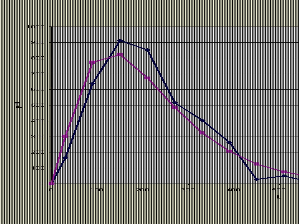
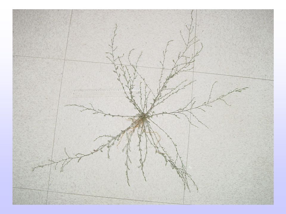
38 Results with a population of trees
The population : 12 apple trees 4 years old grown from the same parents

39

40

41 1. The number of hydraulic lengths,
corresponding to apexes, cannot exceed a few thousand for a given class ; 2. Moreover, the distribution of hydraulic lengths, as well as the distribution of their n components can be more or less influenced by the environment constraints.

42

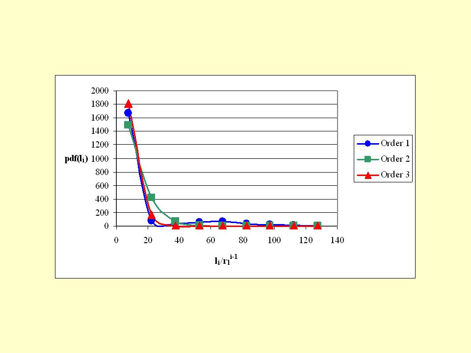
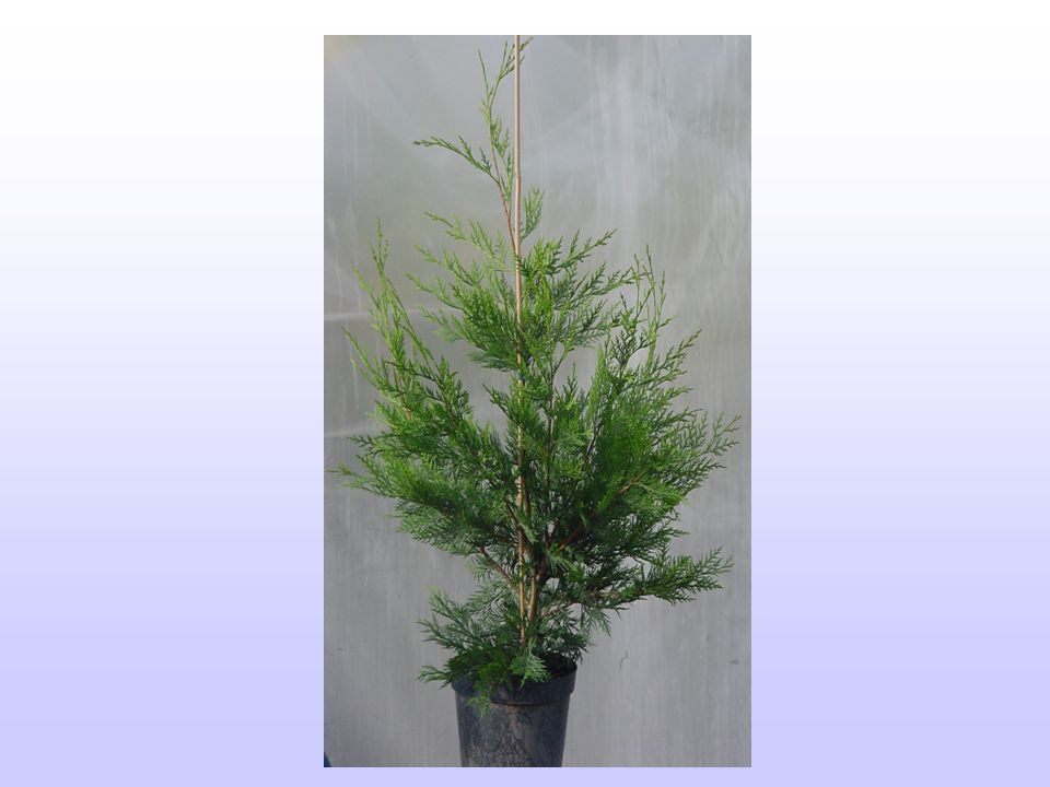
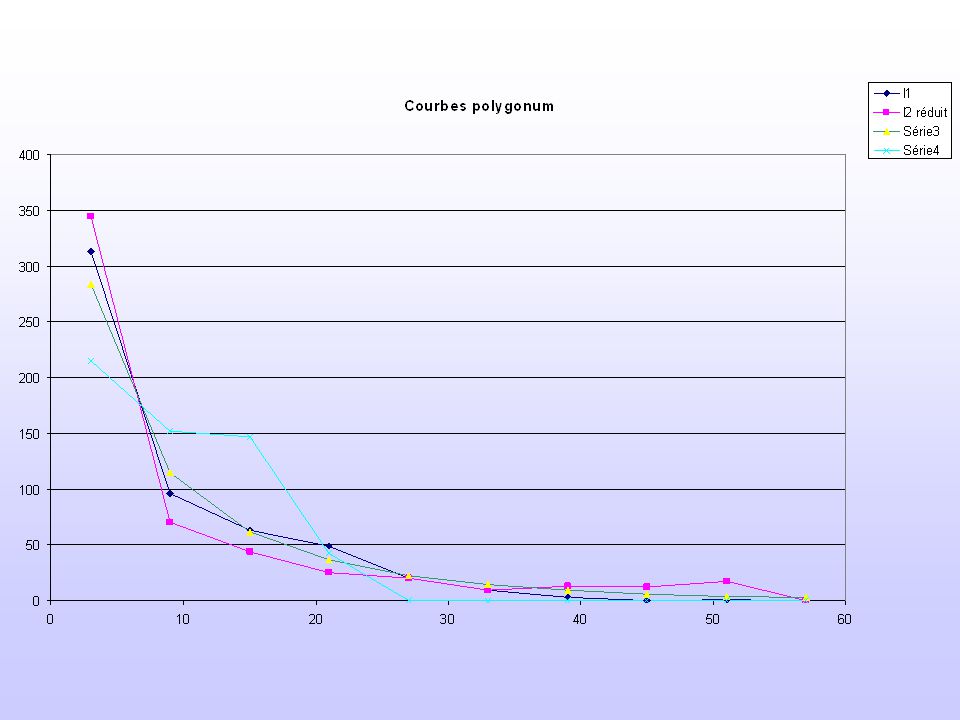
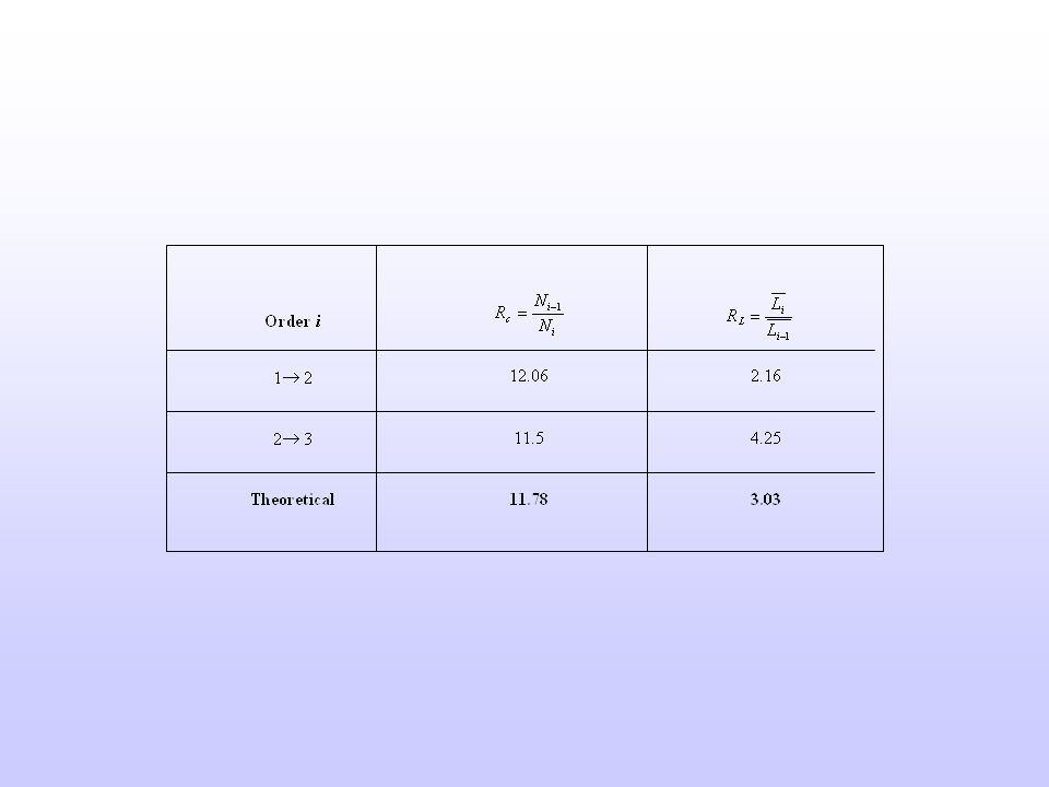
43 Results with a Cupressocyparis
Order n : the maximum order observed in the tree Mean hydraulic length : the average of all the hydraulic lengths of the tree In the same way, RB and RL are calculated for all branches of the tree

44

45

46 Une loi universelle de la morphométrie des arbres ?
Introduction Démonstration de la loi Résultats et discussion Conclusion

47

48

49 Réseaux sur Titan (source : ESA)

50 Biblio sommaire Fleurant C., Duchesne, J., Raimbault, P., An allometric model for trees. Journal of Theorical Biology, 227, Cudennec C., Fouad Y., Sumarjo Gatot I. & Duchesne J A geomorphological explanation of the unit hydrograph concept. Hydrological processes, 18, Duchesne J., Raimbault P. & Fleurant C Towards a universal law of tree morphometry by combining fractal geometry and statistical physics, in Proceeding "Emergent Nature", 7th multidisciplinary conference, M. M. Novak (ed.), World Scientific 2002, pp Roland B An attempt to characterise Hedgerow lattice by means of fractal geometry, , in Proceeding "Emergent Nature", 7th multidisciplinary conference, M. M. Novak (ed.), World Scientific 2002, pp Duchesne, J, Fleurant, C. & Capmarty-Tanguy, F., inventeurs, 2002, Procédé d’implantation de végétaux, plan d’implantation de végétaux obtenu et système informatique pour l’élaboration d’un tel plan, déposé à l’INPI le 25 juin 2002.

51 Merci de votre attention

52

53 This is the density of the points representing the speeds

54 As we have :