Analyse de la variance : ANOVA à un facteur

Présentation au sujet: "Analyse de la variance : ANOVA à un facteur"— Transcription de la présentation:

1 Analyse de la variance : ANOVA à un facteur
Sir Ronald Fischer

2 Thèmes Le modèle linéaire général Les postulats de base
La logique de l’analyse de la variance Exemples Les tests post-hocs La taille d’effet Last week we have discussed the logic of inference statistics in general. Essentially, we try to compare the statistic obtained from our sample to a theoretical sampling distribution that assumes the null hypothesis. Analysis of variane was developed between the two world wars by Sir Ronald R. Fisher to address problems in agriculture. Specifically, to assess whether different fertilizers have different efficiency. For this a number of fields used to be fertilied with different fertilizers and the results observered. Consequently, the techniques was developed for use with discrete independent variables. For continous variables we employ multiple regression.

3 Le modèle général linéaire
Xij - la valeur observée pour le sujet i du groupe j µ - la grande moyenne j - l’influence du traitement sur le groupe j (j = µj - µ) eij - l’erreur ou les résidus - selon les postulats - sont distribués de manière normale avec une moyenne de µ = 0 et un écart-type de . Xij = µ + j + eij Exemple: la taille moyenne des hommes est 68” et la taille moyenne des femmes est 65” La taille d’un homme sera donc: e et la taille d’une femme: e The general linear model has three components: first the grand mean - this is a constant. Ex: differences in size between male and female mice and humans. the grand mean reflects the average size of humans or mice in relation to which we can study the sex difference second the treatment effect: alpha represents the influence on the observed value that is due to the treatment group. If alpha1 = 0 this means that the treatment 1 does not influence the values in that treatment group. If = 0 none of the treatment groups has an influence - that is all means are from the same population finally e describes the error. This includes random meaurement error, but more generally refers to unexplained variance. That is, e might contain a component that is due to a factor which is not included in the model. Since it is not included it remains unexplained and becomes part of the error.

4 Répartition des variances
xij = µ + j + eij avec µ : j : eij : Donc: We will see that the specific logic of the analysis of variance procedure is based on this representation. Specifically, we can calculate the deviation of a specific value xij from the grand mean as: SStot = ∑∑ (xij - X..)2; we also know that xij - X.. = (xij - X.j) + (X.j - X..) consequently we can write: SStot = ∑∑ (xij - X..)2 = ∑∑ (xij - X.j)2 +∑ nj (X.j - X..)2 this actually can be expressed as SStot = SSwithin - SSbet - why? The term ∑∑ xij - X.j expresses the sum of the deviations of each individual value from the mean of the group, that is the variation within the groups. While ∑ X.j - X.. expresses the deviation of the group means from the grand total, that is, the variation between groups. We can calculate the corresponding df for each of these terms. SStot has N-1 degrees of freedom - why? SSwithin has N-J degrees of freedom and SSbetween has J-1 degrees of freedom - why? SStot = ∑∑(aj+eij)2 = nj∑aj 2 + ∑∑eij 2 + 2∑∑ajeij with = 0 and aj 2 =  nj (X.j - X..)2 since a is a constant within each group with assumption that all observations are independently drawn from normal treatment populations with the same variance and indep. errors across all pairs of observations

5 Les sommes des carrés

6 Les postulats de base 1. Le modèle général s’applique aux données
2. Les valeurs sont distribuées normalement dans la population 3. Les échantillons ont des variances homogènes 4. Les échantillons sont indépendants There is one more point to note: the basic assumptions of the analysis of variance. These are: 1. The general linear model is adequate for the data 2. The values are normally distributed in the population 3. The samples have homogenous variances 4. The samples are independant Violation of assumption 1 is untestabl; however its violatio has serious consequences. violation of assumption 4 is easily avoided. Regarding violations of assumptions 2 and 3. As regards assmption 3 we can say that: 1. if the sample sizes are equal violation of this assmption does not lead to problems. ANOVA is robust against this violation. (ratio largest/smallest = 1.5) 2. If sample sizes and variances are unequal and the larger sample has also the smaller variance than the probability of making a Type 1 error is larger than alpha. 3. If sample sizes and variances are unequal and the larger sample has the greater variance than the probability of making a Type 1 error is smaller than alpha. Regarding assumption 2 - normal distribution of the values in the population, we can say that this effect is minial if the sample is relatively large. In sum, for equal cell sizes ANOVA is robust against violations of the basic assumptions regarding homogeneity of variances and normal distribution of values in the population.

7 La logique de l’ANOVA So why does this help us to test the hypothesis that µ1 = µ2 = ... µj = µ ? Lets assume we have four groups such that: Sample population mean variance a A µA I2 b B µB I2 c C µC I2 d D µD I2 Remember that one of the basic assumptions of the analysis of variance procedure is that 12 = 22 = ... = j2 = i2. Conseqently, we can estimate i2 the population variance from the mean of the variances of the four groups. That is, i2 -> 1/N-J ∑∑ (xij - X.)2 which is the same as the SS within divided by their df - this is usually calles mean sums of squares within. In other words the mean sums of squares within is an unbiased estimate of the population variance. This estimate is reliable whether or not the null hypothesis is true, given that we assume homogeneity of variances for all groups. But, under the the condition that the null hypothesis is true - and only under this condition we have another means of estimating the population variance. For this we have to go back to the central limits theorem which states that: if we draw repeated samples from a population with the mean µ and the variance ∂2, then the samples will be normally distributed with a mean of µ and a variance of ∂2 /n. Why does this provide us with another means of estimating the population variance?

8 La logique de l’ANOVA (suite)
Les variances des différents échantillons sont donc égales et elles sont égales à la variance de la population p. 1 = 2 = ... = ij = p avec 1 = s1 = Nous pouvons donc estimer la variance de la population à partir de la moyenne des variances des échantillons ou bien: If the null hypothesis: µ1 = µ2 = ... = µ is true, then all our groups are samples from the same population with the mean µ and the variance 2. This sample has a sampling distribution with a mean = µ and a variance = p2/n. To estimate the population variance we only have to calculate the mean deviation of the sample means from the grand mean and multiply this value by n. In other words, E(sx.2) = E(∑ (X.j - X..)2 /J-1 = x.2 = p2 /n since E(∑ (X. - X..)2 /J-1 = p2 /n but we want to estimate p2 we have to multiply the equation on both sides by n this gives us: nj ∑ (X.j - X..)2 /J-1 which happens to be the mean SS between. The mean square between is an unbiased estimate of the population variance plus a term which is 0 if and only if the null hypothesis is true. We now have two estimates of the population variance which for the case that the null hypothesis is true should give us more or less the same value. That is, if the null hypothesis is true the two estimates should be the same except for the influence of random factors. So all we have to do is to divide the MSSbetween by the MSSwithin, if the null hypothesis is true the resulting value should be somewhere around 1. If the null hypothesis is not true than the resulting value should depart from 1. In this case the MSS between will become larger, while the MSS within will not change (it is not dependent on whether or not the null hypothesis is true) -> F will be larger than 1. The only thing that remains to do is to find a sampling distribution for the quotient. This is the F-distribution. (lets forget how one calculates this distribution). That is, the values for F with a certain number of degrees of freedom. This distribution has two df's the df of the nominator and the denominator. Lets try and go through this procedure step by step for the example above.

9 Selon le théorème des limites centrales: la distribution d’échantillonnage a une moyenne de µ et une variance de 2 /n si l’hypothèse nulle est vraie il suit donc que: pour l’estimé de p 2 il faut multiplier par n

10 Exemple Afin de tester l’hypothèse que la consommation de caféine facilite l’apprentissage trois groupes d’étudiants se préparent à un examen: le groupe 1 boit une tasse, le groupe 2 boit 2 tasses et le groupe 3 boit 3 tasses de café. Voici leurs scores à l’examen:

11 Exemple suite

12 Sommes des carrés moyens
Intra-groupe: Inter-groupe:

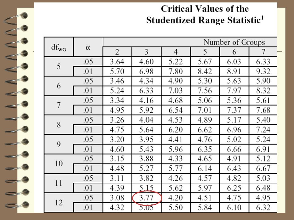
13 Calcul de F Valeur critique pour 2,12 df et a = .05 -> 3.89

14 Exemple 2

15 Suite

16 Sommes des carrés moyens
Intra-groupe: Inter-groupe:

17 Calcul de F Valeur critique pour 2,12 df et a = .05 -> 3.89

18 Tableau ANOVA

19 Résumé La variance intra-groupe (la somme moyenne des écarts carrés entre chaque observation et la moyenne du groupe) est un estimé de la variance de la population. Quand l’hypothèse nulle est vraie - et seulement dans ce cas - la variance inter-groupe (la somme moyenne des écarts carrés entre chaque moyenne de groupe et la grande moyenne) est, selon le théorème des limites centrales, aussi un estimé de la variance de la population Quand il y a un effet de traitement, donc quand l’hypothèse nulle est fausse, la variance inter-groupe est plus large que la variance intra-groupe L’analyse de la variance consiste à calculer le rapport entre la variance inter-groupe et la variance intra-groupe et de comparer le résultat avec une distribution d’échantillonnage connue: la distribution F.

20 Les tests post-hocs

21 Erreurs Erreur (ou ) par comparaison - le niveau  choisi pour une seule comparaison de moyennes Erreur par famille - le nombre moyen des erreurs faites par famille de comparaisons ’  1- (1-)c  C’ Exemple: ’ = .01 et C = 5  = .049 ou approx. .05 In the simplest case we could use a series of t-test to make pairwise comparisions. For example, we could compare x1-x2, x1-x3, x1-x4, x2-x3, x2-x4, x3-x4 in a series of 6 t-tests. However, if we do this we incur a problem. Each of these comparisions will be conducted at a certain alpha level - e.g., That is, each time we conduct the test we will have a .05 chance of making a type 1 error. The more tests we conduct the higher will be the error. In fact lets look at how much higher the error will be. What is the chance of making an error on the first test? on the second ? on either the first or the second .(10)? if we have three tests (.14)? and 6 (.26)? We therefore need to correct for this - Bonferroni However, Bonferroni correction works only on independent comparisions - explain x1-x2=A, x1-x3=B, x2-x3=? x1=A+x2, (A+x2) -x3=B, x2 =B-A+x3, B-A+x3-x3=B-A (see modification de Keppel)

22 Contraste Définition: Une comparaison de J moyennes telle que la différence entre deux des J moyennes ou la différence entre une moyenne et la moyenne de deux autres moyennes c11c22cjjcjj To conduct a post hoc test we have to compare multiple means. This is a general definition. It is important to note that we do not have to compare means one by one - rather we can compare groups of means.

23 Excursion - Orthogonalité
Une comparaison est orthogonale si:  (c1jc2j)/nj= 0 Exemple: jth moyenne C 1: C2: C3: 1 vs 2:  c1jc2j =(1)(1) + (-1)(0) + (0)(-1) + (0)(0) = 1 1 vs 3:  c1jc2j =(1)(0) + (-1)(0) + (0)(1) + (0)(-1) = 0 How do we assess orthogonality? Modification de Keppel:

24 Tukey’s-HSD (John Tukey, 1915-2000)

25

26 La taille d’effet

27 Taille de l’effet La corrélation entre la VI et la VD (r)
Le pourcentage de la variance de la VD expliqué par la VI (r2) La différence entre deux moyennes en unités d’écart-type (d)

28 Taille d’effet: eta2 et omega2

29 Les tailles

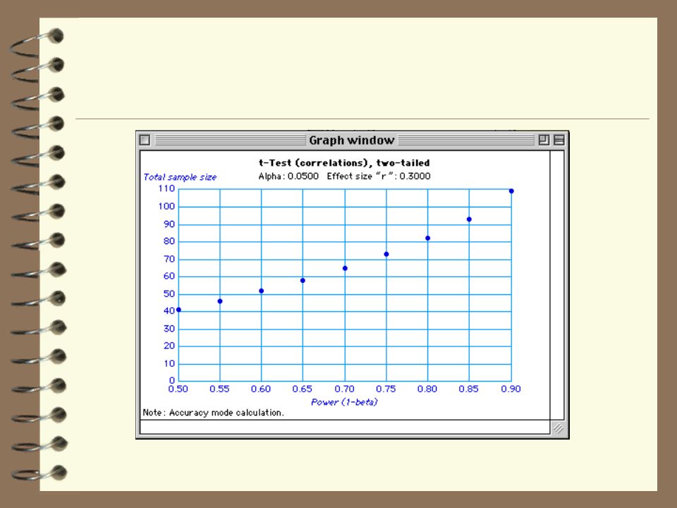
30 Puissance La probabilité de trouver un effet de taille x dans un échantillon de taille N en utilisant un test statistique avec un a donné. Fcrit = 2.58

31 Les erreurs

32 Taille d’effet et beta

33 Variance et beta

34 Calcul de puissance

35 Calcul de puissance

36

37